Reciprocity Applied to Dipole Sources - 1. Near Fields
We continue this series on modelling point dipole sources to discuss applying the principle of reciprocity to dipoles. In this post, we will introduce the concept of reciprocity and apply it to the near fields of dipoles. Future posts will then discuss applying reciprocity to the far fields of dipoles. The following steps are presented in this post,
- Introduction to reciprocity.
- Numerical validation of reciprocity with JCMsuite.
- Using reciprocity to eliminate a source.
The Lorentz Reciprocity Theorem
The following theoretical background is based on this page/10%3A_Antennas/10.10%3A_Reciprocity), take a look there for a more in depth mathematical treatment of the theorem.
The reciprocity theorem is a fundamental concept in the field of electrical engineering and electromagnetic theory. It relates to the behaviour of electromagnetic fields in linear, time-invariant systems and establishes a relationship between two aspects: the excitation and response of a system when considering the interchange of source and observation points. In simpler terms, it states that the electromagnetic fields produced by a source at one location are the same as the fields observed at another location when the roles of the source and observation points are swapped.

Basic Principle
The reciprocity theorem is based on the basic principle that in linear, time-invariant systems, the behaviour of electromagnetic fields should remain the same when you swap the roles of the source and observation points while keeping the source and the surrounding medium unchanged.
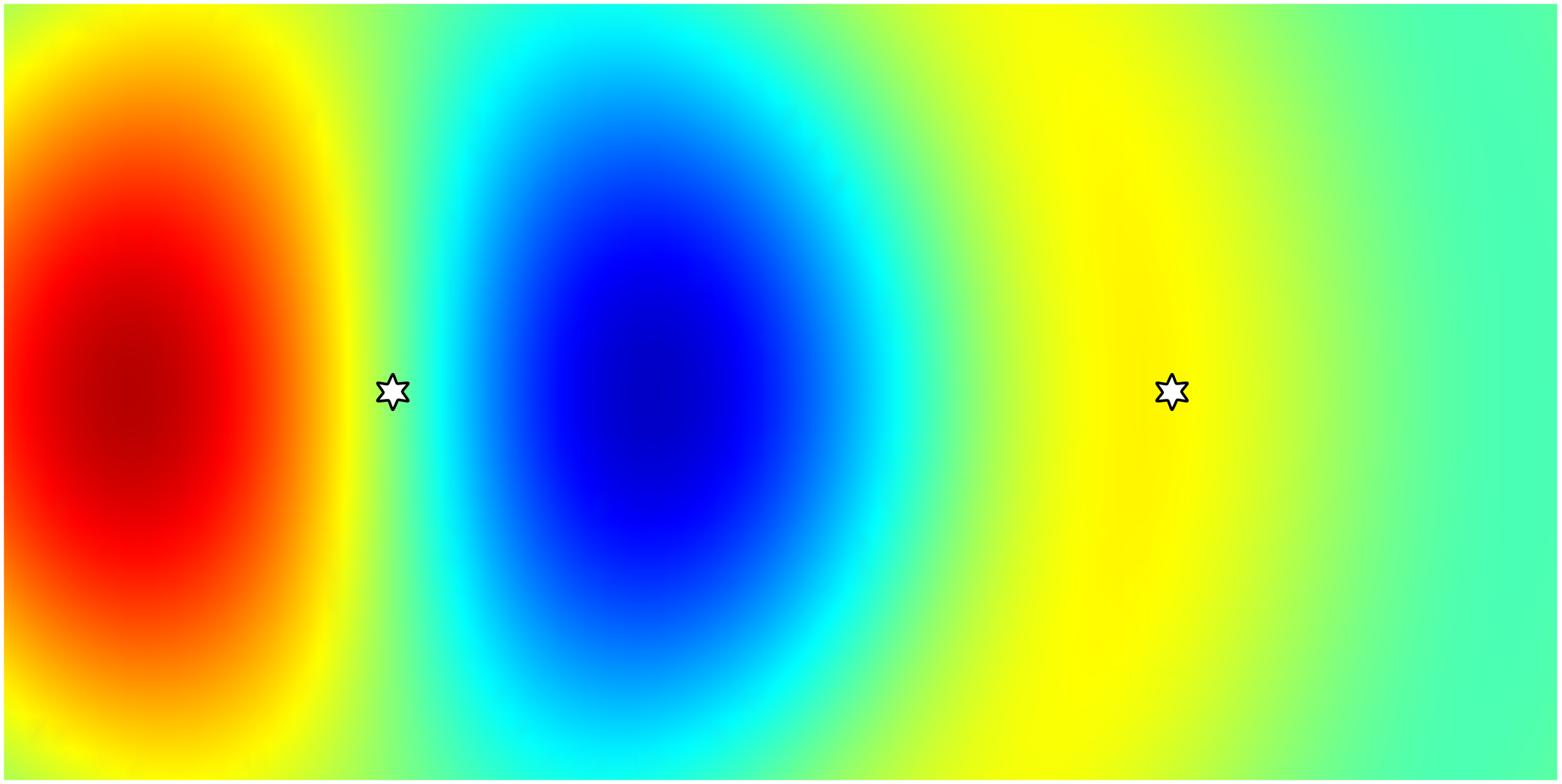
As an example, take the two dipole sources $\mathrm{\mathbf{J}}_{1}$ and $\mathrm{\mathbf{J}}_{2}$ and their associated electric fields $\mathrm{\mathbf{E}}_{1}$ and $\mathrm{\mathbf{E}}_{2}$ shown in figure 1. The two dipoles are located at positions $\mathrm{\mathbf{r}}_{1}$ and $\mathrm{\mathbf{r}}_{2}$. the reciprocity theorem states that:
Putting this into a mathematical formulation:
\begin{equation} \int_{V} {\left[\mathrm{\mathbf{J}}_{1}(\mathbf{r}) \cdot \mathrm{\mathbf{E}}_{2}(\mathbf{r}) - \mathrm{\mathbf{J}}_{2}(\mathbf{r}) \cdot \mathrm{\mathbf{E}}_{1}(\mathbf{r})\right] dv}. \end{equation}Here the subscripts indicate which source is being referenced. Although this expression is valid for any two non-overlapping current density distributions, it is further simplified when using point dipole sources. These have the following form $\mathrm{\mathbf{J}(\mathbf{r}, t)} = \mathrm{\mathbf{j}}\delta (\mathbf{r}-\mathbf{r_{0}})e^{-i\omega t}$ which simplifies the integral to an algebraic expression,
\begin{equation} \mathrm{\mathbf{j}}_{1} \cdot \mathrm{\mathbf{E}}_{2}(\mathbf{r}_{1}) = \mathrm{\mathbf{j}}_{2} \cdot \mathrm{\mathbf{E}}_{1}(\mathbf{r}_{2}). \end{equation}Verification with JCMsuite
To demonstrate the principle of reciprocity, we can simulate a setup similar to figure 1 in JCMsuite. Two dipole sources are spaced 500 nm apart, emitting both at a wavelength of 450 nm. The dipoles have polarization vectors $\mathrm{\mathbf{j}}_{1} = [0, 1, 0]$ Am$^{-2}$ and $\mathrm{\mathbf{j}}_{2} = [0, 1, 1]$ Am$^{-2}$. We also use the ExportFields post process to obtain the resulting electric fields at both dipole positions.
Knowing the input source current densities and their associated field strengths, we can verify the reciprocity theorem:
import os, sys
import numpy as np
from scipy import constants

sys.path.insert(0,os.path.join(os.getenv('JCMROOT'), 'ThirdPartySupport', 'Python'))
import jcmwave as jcm

source_dir = os.path.join(".","sources")
# the current density vectors
j1_r1 = np.array([0, 1, 0])
j2_r2 = np.array([0, 1, 1])
# load the efield results from the JCMsuite post process output
e_field = jcm.loadtable(os.path.join(source_dir,"two_isolated_dipoles","project_results","efield.jcm"))
e1_r2 = e_field['ElectricFieldStrength'][0][1, :]
e2_r1 = e_field['ElectricFieldStrength'][1][0, :]

#j1.e2 = j2.e1
print("proof of reciprocity theorem:")
lhs = np.dot(j1_r1, e2_r1)
rhs = np.dot(j2_r2, e1_r2)
print(f"left-hand side: \t\t\t{lhs}")
print(f"right-hand side: \t\t\t{rhs}")
print(f"relative error on real part: \t\t{np.abs(np.real((lhs-rhs)))/np.abs(np.real(rhs)):.5e}")
print(f"relative error on imaginary part: \t{np.abs(np.imag((lhs-rhs)))/np.abs(np.imag(rhs)):.5e}")
Using Reciprocity to Eliminate one Source
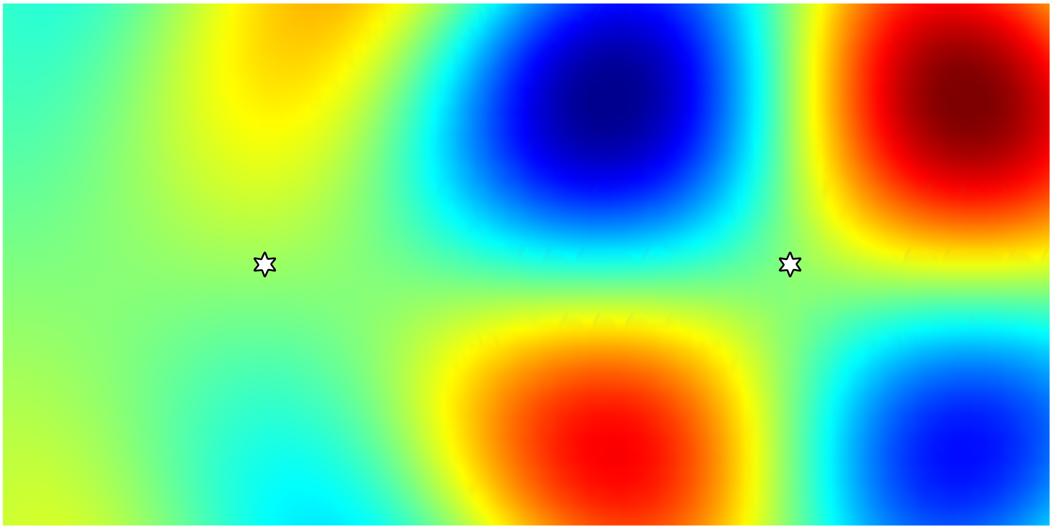
Suppose now that our goal is to calculate the electric field at position two $\mathrm{\mathbf{E}_{1}(\mathbf{r}_{2})}$ due to a source at position one $\mathrm{\mathbf{j}_{1}(\mathbf{r}_{1})}$, as shown here,

Instead of placing a dipole at $\mathrm{\mathbf{r}_{1}}$, we wish to obtain the result using reciprocity. To show how this is done, it can be helpful to expand the reciprocity equation in full,
\begin{equation} \mathrm{\mathbf{j}}_{1} \cdot \mathrm{\mathbf{E}}_{2} = \mathrm{\mathbf{j}}_{2} \cdot \mathrm{\mathbf{E}}_{1} , \\ \mathrm{j}_{1,x}\mathrm{E}_{2,x} + \mathrm{j}_{1,y}\mathrm{E}_{2,y} + \mathrm{j}_{1,z}\mathrm{E}_{2,z} = \mathrm{j}_{2,x}\mathrm{E}_{1,x} + \mathrm{j}_{2,y}\mathrm{E}_{1,y} + \mathrm{j}_{2,z}\mathrm{E}_{1,z}. \end{equation}
Since we have free reign over the value of the source $\mathrm{\mathbf{j}_{2}(\mathbf{r}_{2})}$ (remember, we are interested in the response of the source $\mathrm{\mathbf{j}_{1}(\mathbf{r}_{1})}$), we choose to simulate for three values of $\mathrm{\mathbf{j}_{2}(\mathbf{r}_{2})}$, namely $\mathbf{\alpha} = [1, 0, 0]$, $\mathbf{\beta} = [0, 1, 0]$ and $\mathbf{\gamma} = [0, 0, 1]$.

This simplifies the previous expression providing three equations to obtain the components of $\mathrm{\mathbf{E}_{1}(\mathbf{r}_{2})}$,
\begin{equation} \mathrm{E}_{1,x} = \frac{1}{\alpha_{x}} (\mathrm{j}_{1,x}\mathrm{E}^{\alpha}_{2,x} + \mathrm{j}_{1,y}\mathrm{E}^{\alpha}_{2,y} + \mathrm{j}_{1,z}\mathrm{E}^{\alpha}_{2,z} ), \\ \mathrm{E}_{1,y} = \frac{1}{\beta_{y}} (\mathrm{j}_{1,x}\mathrm{E}^{\beta}_{2,x} + \mathrm{j}_{1,y}\mathrm{E}^{\beta}_{2,y} + \mathrm{j}_{1,z}\mathrm{E}^{\beta}_{2,z} ), \\ \mathrm{E}_{1,z} = \frac{1}{\gamma_{z}} (\mathrm{j}_{1,x}\mathrm{E}^{\gamma}_{2,x} + \mathrm{j}_{1,y}\mathrm{E}^{\gamma}_{2,y} + \mathrm{j}_{1,z}\mathrm{E}^{\gamma}_{2,z} ). \end{equation}
Where the superscripts for the electric field refer to a specific value of the source $\mathrm{\mathbf{j}_{2}(\mathbf{r}_{2})}$. Due to our choice of $\alpha_{x} = \beta_{y} = \gamma_{z} = 1$, this further simplifies to,
\begin{equation} \mathrm{E}_{1,x} = (\mathrm{j}_{1,x}\mathrm{E}^{\alpha}_{2,x} + \mathrm{j}_{1,y}\mathrm{E}^{\alpha}_{2,y} + \mathrm{j}_{1,z}\mathrm{E}^{\alpha}_{2,z} ), \\ \mathrm{E}_{1,y} = (\mathrm{j}_{1,x}\mathrm{E}^{\beta}_{2,x} + \mathrm{j}_{1,y}\mathrm{E}^{\beta}_{2,y} + \mathrm{j}_{1,z}\mathrm{E}^{\beta}_{2,z} ), \\ \mathrm{E}_{1,z} = (\mathrm{j}_{1,x}\mathrm{E}^{\gamma}_{2,x} + \mathrm{j}_{1,y}\mathrm{E}^{\gamma}_{2,y} + \mathrm{j}_{1,z}\mathrm{E}^{\gamma}_{2,z} ). \end{equation}
Therefore, we can reconstruct the value of $\mathrm{\mathbf{E}_{1}(\mathbf{r}_{2})}$ using the three values of $\mathrm{\mathbf{E}_{2}(\mathbf{r}_{1})}$ from the three different sources $\mathrm{\mathbf{j}_{2}(\mathbf{r}_{2})}$, combined with the value of the source for which we want to calculate the response $\mathrm{\mathbf{j}_{1}(\mathbf{r}_{1})}$.
Example with JCMsuite
# the current density vector
j1_r1 = np.array([1, 2, 3])

# load the efield results from the JCMsuite post process output
e_field = jcm.loadtable(os.path.join(source_dir, "isolated_dipole_via_reciprocity", "project_results", "efield.jcm"))

e2_r1_xpol = e_field['ElectricFieldStrength'][0][0, :]
e2_r1_ypol = e_field['ElectricFieldStrength'][1][0, :]
e2_r1_zpol = e_field['ElectricFieldStrength'][2][0, :]

e1_r2 = e_field['ElectricFieldStrength'][3][1, :]

e1_r2_xpol = np.dot(e2_r1_xpol, j1_r1)
e1_r2_ypol = np.dot(e2_r1_ypol, j1_r1)
e1_r2_zpol = np.dot(e2_r1_zpol, j1_r1)

e1_r2_recip = np.array([e1_r2_xpol, e1_r2_ypol, e1_r2_zpol])


norm = np.linalg.norm(e1_r2)

# showing e2_r1 and e2_r1_recip are equivalent:

print(f"x component relative error: {np.abs(e1_r2[0]-e1_r2_recip[0])/norm:.8e}")
print(f"y component relative error: {np.abs(e1_r2[1]-e1_r2_recip[1])/norm:.8e}")
print(f"z component relative error: {np.abs(e1_r2[2]-e1_r2_recip[2])/norm:.8e}")
Conclusion
The reciprocity theorem is a powerful tool for simplifying electromagnetic simulations. In this post we have introduce the basic concepts of using reciprocity and verify them numerically.
In particular, we presented the following examples:
- Reciprocity applied to simulating two dipoles near to each other.
- Eliminating a dipole source by simulating three linearly independent sources at a different position.
The next post in this series will go on to discuss applying reciprocity to dipoles in the far field. In that case, the elimintion of sources presented here can be a great benefit computationally.
Additional Resources
- Download a free trial version of JCMsuite.
- Documentation for dipole sources in JCMsuite can be found here.
- Documentation for export field post process in JCMsuite can be found here
- Mathematical Background of the Reciprocity Theorem/10%3A_Antennas/10.10%3A_Reciprocity)